


Introduction
I would highly recommend you check out Mnist handwritten digit classification using tensorflow before continuing with this article. In that article, I tackled the same MNIST handwritten digit classification using a simple neural network.
Convolutional Neural Networks (CNNs) are the current state-of-art architecture mainly used for the image classification tasks. They are also known as shift invariant or space invariant artificial neural networks, what this means is that even if the digit in the image is not in the exact spot as in the training we will still be able to correctly classify the image.
They have applications in image and video recognition, recommender systems, image classification, image segmentation, medical image analysis, natural language processing, brain-computer interfaces, and financial time series.
CNN's are regularized versions of multilayer perceptrons. Multilayer perceptrons usually mean fully connected networks, that is, each neuron in one layer is connected to all neurons in the next layer.
enough chit chat, let's dive right in
Importing the modules
Required packages are -
- Tensorflow
- matplotlib
- numpy
- jupyter
- opencv
import tensorflow as tf

# Loading the dataset
mnist = tf.keras.datasets.mnist

# Divide into training and test dataset
(x_train, y_train),(x_test, y_test) = mnist.load_data()

x_train.shape
# (60000, 28, 28)
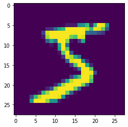
Hence training data contains 60,000 images. Each of these images is 28 pixels wide and 28 pixels high
import matplotlib.pyplot as plt
plt.imshow(x_train[0])
plt.show()
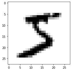
The image in the dataset is a colour image, we can convert it into greyscale using matplotlib's build-in colour map.
plt.imshow(x_train[0], cmap = plt.cm.binary)
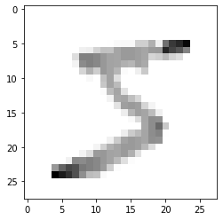
Normalization
The original image is black and white but the value ranges from [0-255]. 0 being the absolute black and 255 being absolute white. But for training, we have to convert this into [0-1].
x_train = tf.keras.utils.normalize(x_train, axis = 1)
x_test = tf.keras.utils.normalize(x_test, axis = 1)
plt.imshow(x_train[0], cmap = plt.cm.binary)
# verify that there is a proper label for the image
print(y_train[0])
# 5
Resizing image for Convolution
You always have to give a 4D array as input to the CNN.
So input data has a shape of (batch_size, height, width, depth), where the first dimension represents the batch size of the image and the other three dimensions represent dimensions of the image which are height, width, and depth.
For some of you who are wondering what is the depth of the image, it’s nothing but the number of colour channels. For example, an RGB image would have a depth of 3, and the greyscale image would have a depth of 1.
In our case, as we are dealing with the greyscale images we can add a depth of 1.
import numpy as np
IMG_SIZE=28
# -1 is a shorthand, which returns the length of the dataset
x_trainr = np.array(x_train).reshape(-1, IMG_SIZE, IMG_SIZE, 1)
x_testr = np.array(x_test).reshape(-1, IMG_SIZE, IMG_SIZE, 1)
print("Training Samples dimension", x_trainr.shape)
print("Testing Samples dimension", x_testr.shape)
# Training Samples dimension (60000, 28, 28, 1)
# Testing Samples dimension (10000, 28, 28, 1)
Creating a Deep Neural Network
- Sequential - A feedforward neural network
- Dense - A typical layer in our model
- Dropout - Is used to make the neural network more robust, by reducing overfitting
- Flatten - It is used to flatten the data for use in the dense layer
- Conv2d - We will be using a 2-Dimensional CNN
- MaxPooling2D - Pooling mainly helps in extracting sharp and smooth features. It is also done to reduce variance and computations. Max-pooling helps in extracting low-level features like edges, points, etc. While Avg-pooling goes for smooth features.
from tensorflow.keras.models import Sequential
from tensorflow.keras.layers import Dense, Dropout, Activation, Flatten, Conv2D, MaxPooling2D

# Creating the network
model = Sequential()

### First Convolution Layer
# 64 -> number of filters, (3,3) -> size of each kernal,
model.add(Conv2D(64, (3,3), input_shape = x_trainr.shape[1:])) # For first layer we have to mention the size of input
model.add(Activation('relu'))
model.add(MaxPooling2D(pool_size=(2,2)))

### Second Convolution Layer
model.add(Conv2D(64, (3,3)))
model.add(Activation('relu'))
model.add(MaxPooling2D(pool_size=(2,2)))

### Third Convolution Layer
model.add(Conv2D(64, (3,3)))
model.add(Activation('relu'))
model.add(MaxPooling2D(pool_size=(2,2)))

### Fully connected layer 1
model.add(Flatten())
model.add(Dense(64))
model.add(Activation("relu"))

### Fully connected layer 2
model.add(Dense(32))
model.add(Activation("relu"))

### Fully connected layer 3, output layer must be equal to number of classes
model.add(Dense(10))
model.add(Activation("softmax"))
we determine the number of filters based on the complexity of the task.
After each layer the filters increases. This is because of how CNN works. After each layer, more complex features are detected and for it, more filters are used.
For example - Taking the example of our MNIST dataset. In the first layer, the filter will be responsible for edge detection, then it can detect curves or circles, like this after each layer it goes on detecting bigger features.
In case of binary classification, sigmoid activated in recommended
Use the below piece of code to better understand the neural network.
model.summary()
Compile defines the loss function, the optimizer and the metrics.
model.compile(loss="sparse_categorical_crossentropy", optimizer="adam", metrics=['accuracy'])
Training the model
model.fit(x_trainr, y_train, epochs=5, validation_split = 0.3)
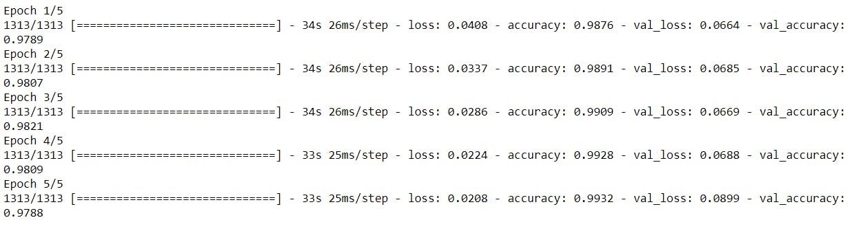
if validation accuracy < accuracy, then the model might be overfitting. So the aim is to make validation accuracy and accuracy almost similar. In case of overfitting, we should try adding dropout layers.
# Evaluating the accuracy on the test data
test_loss, test_acc = model.evaluate(x_testr, y_test)
print("Test Loss on 10,000 test samples", test_loss)
print("Test Accuracy on 10,000 test samples", test_acc)

predictions = model.predict([x_testr])
print(predictions)
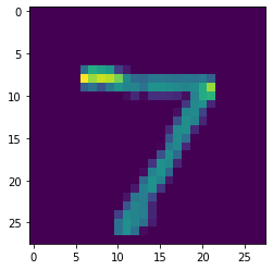
plt.imshow(x_test[0])
print(np.argmax(predictions[0]))
# 7
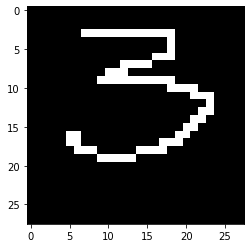
Checking on our on input images
I created an image with number in windows paint.
import cv2
img = cv2.imread('three.png')
plt.imshow(img)
img.shape
# (28, 28, 3)

# Converting to grayscale
gray = cv2.cvtColor(img, cv2.COLOR_BGR2GRAY)
gray.shape
# (28, 28)

# Resizing to a 28x28 image
# Please note my image was already in correct dimension
resized = cv2.resize(gray, (28,28), interpolation = cv2.INTER_AREA)
resized.shape
# (28, 28)

# 0-1 scaling
newimg = tf.keras.utils.normalize(resized, axis = 1)

# For kernal operations
newimg = np.array(newimg).reshape(-1, IMG_SIZE, IMG_SIZE, 1)

newimg.shape
# (1, 28, 28, 1)

predictions = model.predict(newimg)
print(np.argmax(predictions[0]))
# 3
Hence, our CNN model was able to correctly identify the number.
Saving the model
# Saving a Keras model:
model.save('path/to/location')
Inorder to use the saved model run the below code
# Loading the model back:
from tensorflow import keras
model = keras.models.load_model('path/to/location')
Conclusion
CNN classifier is really powerful. We were able to correctly identify the number. When compared to the MNIST using simple neural network we got much better accuracy and this model can handle a wide variety of input images too.
Thanks for reading.